The models we studied in Chapter 5 treat the variable of interest as dependent on its own past, and possibly on a set of exogenous variables. While this approach is useful, often, economic and financial variables may interact simultaneously rather than in isolation. For example, GDP and consumption influence each other, as do interest rates and inflation, stock returns and exchange rates, industrial production and trade flows, or sales and prices. These relationships are inherently dynamic, bidirectional, and endogenous, meaning that variables mutually influence one another. As a result, relying on a single equation model unrealistically forces the analyst to designate one variable as dependent and treat the others as exogenous. A vector Autoregression (VAR) treats all variables as endogenous. Instead of modeling one equation, we can model a system of equations where each variable depends on its own lags and the lags of all other variables. Formally:
A Vector AutoRegression (VAR) is a set of k time series regressions, in which the regressors are lagged values of all k series. With \(p\) number of lags in each of the equations is the system of equations is called a \(VAR(p)\). For \(k=2\):
In a VAR with \(k\) variables and \(p\) lags, each equation includes \(k \times p\) regressors. You estimate \(k\) separate regressions, so the system becomes a collection of standard linear regressions with identical regressors.
For instance, a VAR(1) with two variables (\(k=2\)) can be expressed as:
Stationarity. Transform the data if needed so that the \(k\) series are stationary. It will be discussed further when studying cointegration.
White noise errors
No perfect multicollinearity
Contemporaneous correlation is allowed. Errors across equations can be correlated.
Variables in the system should be plausibly related, so they can meaningfully help forecast one another. Including unrelated variables adds estimation noise without contributing predictive information, ultimately reducing forecast accuracy.
The choice of lag lengths is also fundamental, we’d like to specify models with the ability to capture the dynamic relationships among variables while maintaining parsimony. As studied earlier, information criteria is useful for this purpose, by extending the single-equation information criterion, AIC or BIC, to a system of equations, the optimal lag length is the one that minimizes the criterion. The selection, however, should be complemented with residual diagnostics (e.g., Ljung-Box test) and interpretability, asking ourselves if the lag length make sense given the frequency of the data.
The Stability Condition
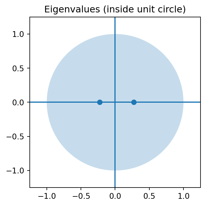
The stability condition requires all the eigenvalues of the coefficient matrix to lie inside the unit circle. The coefficient matrix in a VAR indicates how variables affect each other over time. The eigenvalues of this matrix then capture the persistence of the system:
Eigenvalues close to 1 \(\rightarrow\) highly persistent dynamics
Eigenvalues greater than 1 \(\rightarrow\) explosive behavior
Eigenvalues less than 1 \(\rightarrow\) stable, mean-reverting system
In other words, each eigenvalue must have modulus less than 1. To better understand the concept, we may think of eigenvalues as measuring how strongly shocks propagate through the system.
The key object is \(\phi^h\). If \(|\phi|<1\), then \(\phi^h \rightarrow 0\) as \(h \rightarrow \infty\), shocks die out. If \(|\phi| \ge 1\), then shocks persist or explode. This is why stationarity in the AR(1) process requires \(∣\phi∣<1\).
They key now is \(A^h\), does \(A^h \rightarrow 0\) as \(h \rightarrow \infty\)?. The matrix \(A\) in a VAR system summarizes two key features of the dynamics, (1) the directions in which the system evolves, captured by the eigenvectors, and (2) the persistence of those dynamics, captured by the eigenvalues. If all eigenvalues have modulus less than 1, then \(A \rightarrow 0\), but if any eigenvalue has modulus \(\ge 1\), \(A^h\) does not decay.
Each eigenvalue tells us how shocks evolve along its corresponding direction. If the modulus of all eigenvalues is less than one, shocks die out over time and the system is stable (stationary).
While stability means that all eigenvalues, \(\lambda_i\) of the companion matrix must satisfy be \(<1\), sometimes statistical software reports the roots, not the eigenvalues directly. These roots are the inverse of the eigenvalues: \(z_i = \frac{1}{\lambda_i}\), so the condition \(\lambda<1\) is equivalent to, roots outside the unit circle, \(z_i >1\).
In short, stability is the multivariate extension of stationarity, it ensures that the system behaves well over time and that the statistical properties needed for inference and forecasting are valid, ensuring that:
Shocks to the system do not explode over time
The effect of shocks gradually dies out
The series fluctuate around a constant mean and variance
NoteExample
Show code
import pandas as pdimport numpy as npimport matplotlib.pyplot as pltimport seaborn as snsimport statsmodels.api as smimport plotly.graph_objects as goimport yfinance as yffrom statsmodels.tsa.api import VARfrom datetime import datetimefrom pandas_datareader import data as pdrfrom statsmodels.tsa.stattools import adfuller, kpssfrom statsmodels.graphics.tsaplots import plot_acf, plot_pacffrom statsmodels.stats.diagnostic import acorr_ljungbox
/var/folders/wl/12fdw3c55777609gp0_kvdrh0000gn/T/ipykernel_45961/2165326570.py:2: InterpolationWarning:

The test statistic is outside of the range of p-values available in the
look-up table. The actual p-value is greater than the p-value returned.
/var/folders/wl/12fdw3c55777609gp0_kvdrh0000gn/T/ipykernel_45961/277256259.py:2: InterpolationWarning:

The test statistic is outside of the range of p-values available in the
look-up table. The actual p-value is greater than the p-value returned.
Estimation
var_data = ts[['gGDP', 'cUnem']]model = VAR(var_data) # Prepares the structure of a VAR modellag_selection = model.select_order(maxlags=8)print(lag_selection.summary())
FPE criterion measures how well the model that is expected to produce out-of-sample forecast error. The lowest value signals the smallest error. HQIC balances fit and parsimony, sitting between AIC and BIC in how strongly it penalizes model complexity.
The model with lag = 0 represents a model with no dynamics. It is included by default to verify that adding lags actually improves the model. Most criteria here select one lag.
p = lag_selection.selected_orders['aic'] # or 'bic', etc.results = model.fit(p)print(results.summary())
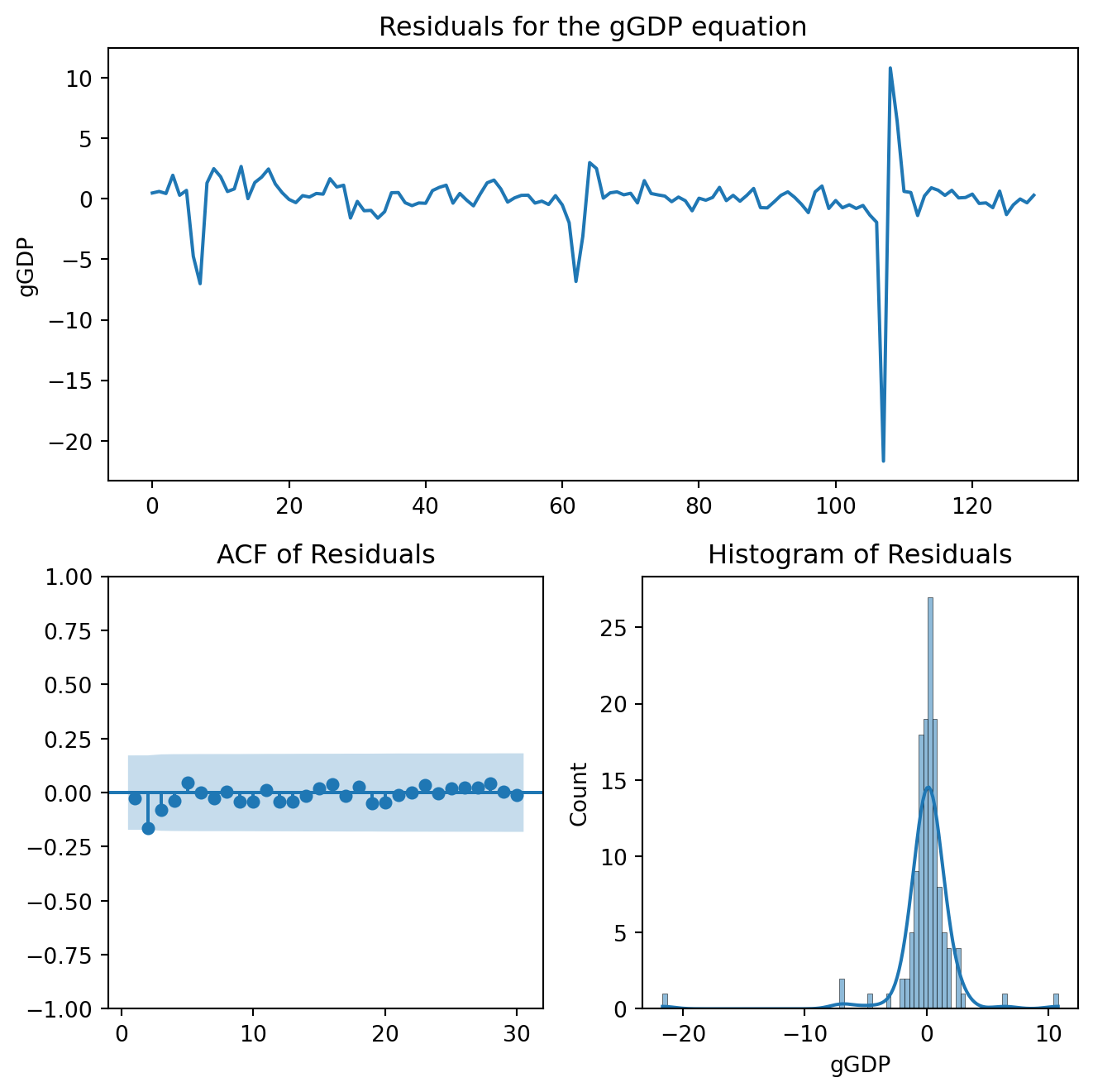
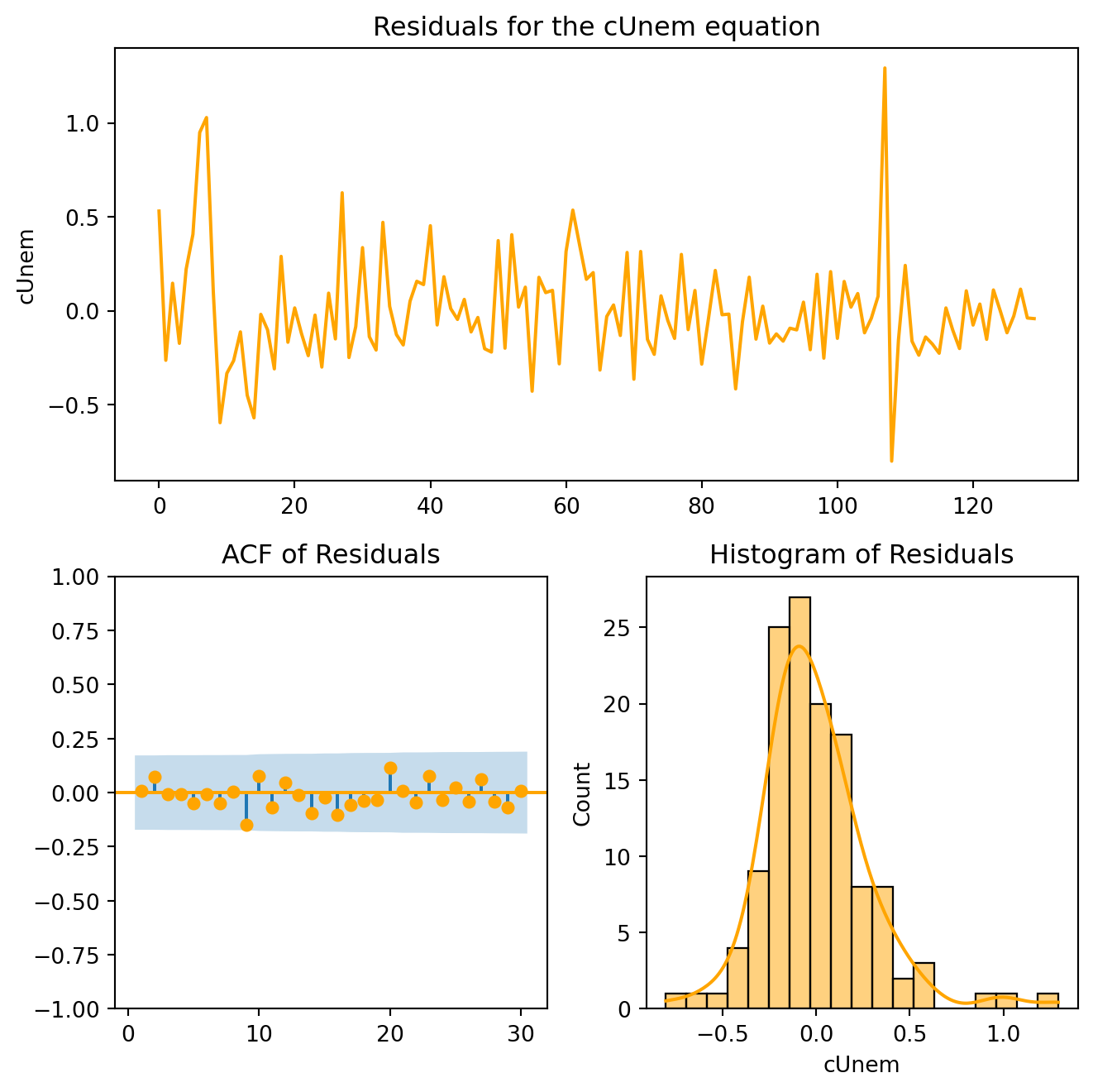
At a 95% confidence level, the null hypothesis of no serial correlation can’t be rejected.
Note that, in principle, the Ljung-Box test should adjust for all dynamic parameters that capture serial dependence in the residuals. In a VAR, this could be captured by the number of lagged regressors in each equation. In practice, some implementations simplify this adjustment, but for consistency with SARIMA models, we counted the number of coefficients for the lagged variables.
The constant (0.565) indicates an average quarterly growth around 0.6%. The coefficient on lagged GDP (-0.19, p = 0.066), implies a negative relationship, growth spikes are often followed by a decrease, a reversion to the mean. Changes in unemployment do not predict GDP growth as the coefficient is not statistically different from zero.
The constant is not statistically different from zero, i.e., we cannot reject the hypothesis that the mean change in unemployment is zero. Over time, unemployment does not trend upward or downward systematically. The coefficient on lagged GDP (-0.025), suggest that higher GDP growth reduces unemployment next period. This is an important result consistent Okun’s Law. What does the coefficient on lagged unemployment indicate?
Once a VAR has been estimated, passed the residual diagnostics, and satisfied the stability condition, we can use it either for predictive purposes or to examine relationships among the variables (or both).
6.1.1 Forecasting
The VAR provides a law of motion for the system that can be used to generate joint forecasts of all variables in which each variable is forecast using its own past and the past of all other variables.
Once the parameters have been estimated, forecasting is obtained by replacing future unknown values with their model-implied expectations conditional on the information available at the forecast origin. Suppose the last observed period is \(T\). The one-period forecast of the system is
\[
\hat{Y}_{T+1|T} = \hat{c} + \hat{A_1}Y_{T} + \hat{A_2}Y_{T-1} + \cdots + + \hat{A_p}Y_{T-p+1}
\] the forecast uses only the deterministic part implied by the estimated model because the expected value of the future innovation is zero.
The multi-period forecast follows the same logic, but now a recursion appears. The two-period forecast is
since \(Y_{T+1}\) is not observed at \(T\), it was replaced by the forecast obtained in the previous step. This recursive structure continues for longer horizons.
Important, stability was required in order to ensure that the forecast path is well behaved. In a stable VAR, the effect of shocks will diminish over time, by contrast, forecasts may explode or behave erratically in an unstable VAR, which is why such a model is not suitable for forecasting or for substantive interpretation.
periods =4forecast = results.forecast(var_data.values[-p:], steps= periods)
VAR models allow us to describe how economic systems respond to shocks. This is the purpose of impulse response analysis. In its moving average representation, the VAR model can be written as:
\(\Phi_h\): describes how shocks propagate over time
Thus, the current value of the system can be interpreted as the accumulation of past shocks and their dynamic effects.
An Impulse Response Function (IRF) traces the effect of a one time shock to one variable on the entire system over time. It allows us to understand how a shock today affects each variable in the system, the direction and magnitude of the response, and how persistent the effect is.
A key complication arises because the residuals, by construction, are correlated, \(Cov(\epsilon_t) = \Sigma \ne I\). As a result, a shock to one equation is not isolated, making interpretation difficult. To address this, we transform the residuals as: \[\epsilon_t = P u_t\] where \(u_t\) is the vector of orthogonal shocks (uncorrelated) and \(P\) is a matrix such that \(PP'=\Sigma\).
This transformation allows us to interpret shocks as independent innovations. Substituting into the Moving Average Representation of the VAR system:
where: \(\Psi_h=\Phi_hP\). Each \(\Psi_h\) describes the response of the system at horizon \(h\) to a one-unit orthogonal shock to one variable, holding shocks to all other variables equal to zero.
Each column of \(\Psi_h\) corresponds to a specific shock, specifically, column \(i\) is the response to a shock in variable \(i\). The rows represent the responses of all variables in the system.
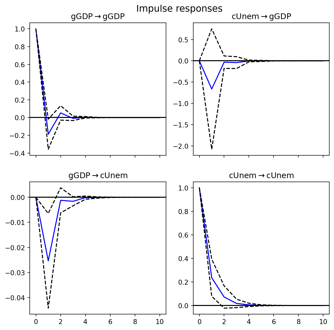
The impulse response functions for our model are obtained as follows:
Each figure in the panel shows how one variable responds over time to a one-time shock in another variable. The horizon tells us how long the effect lasts.
Suppose Mexico experiences a sudden surge in manufacturing exports due to nearshoring demand from the U.S., stronger than anticipated, how does unemployment respond over the next quarters?
NotePractice
Apply Vector Autoregression (VAR) techniques to analyze the dynamic interaction between long-term interest rates and market uncertainty. Using data on the 10-year U.S. Treasury yield and the VIX index, this exercise explores how changes in financial conditions and perceived risk evolve jointly over time. Understanding the relationship between interest rates and volatility is essential in finance, as shifts in risk sentiment and term structure dynamics influence asset pricing, portfolio allocation, and hedging strategies.
We will estimate a VAR model, select the appropriate lag length, and evaluate its adequacy through diagnostic and stability tests. Finally, impulse response functions will be used to examine how unexpected changes in long-term yields affect market volatility, and vice versa. The goal of the exercise is to move beyond model estimation and develop the ability to interpret dynamic relationships in financial markets in a rigorous and economically meaningful way.
6.2 Cointegration
If we regress one nonstationary series on another, we may obtain apparently strong results even when the variables are unrelated. This is the problem of spurious regression and a reason why we have emphasized the importance of testing for unit roots and, when needed, transforming the data by taking differences before modeling.
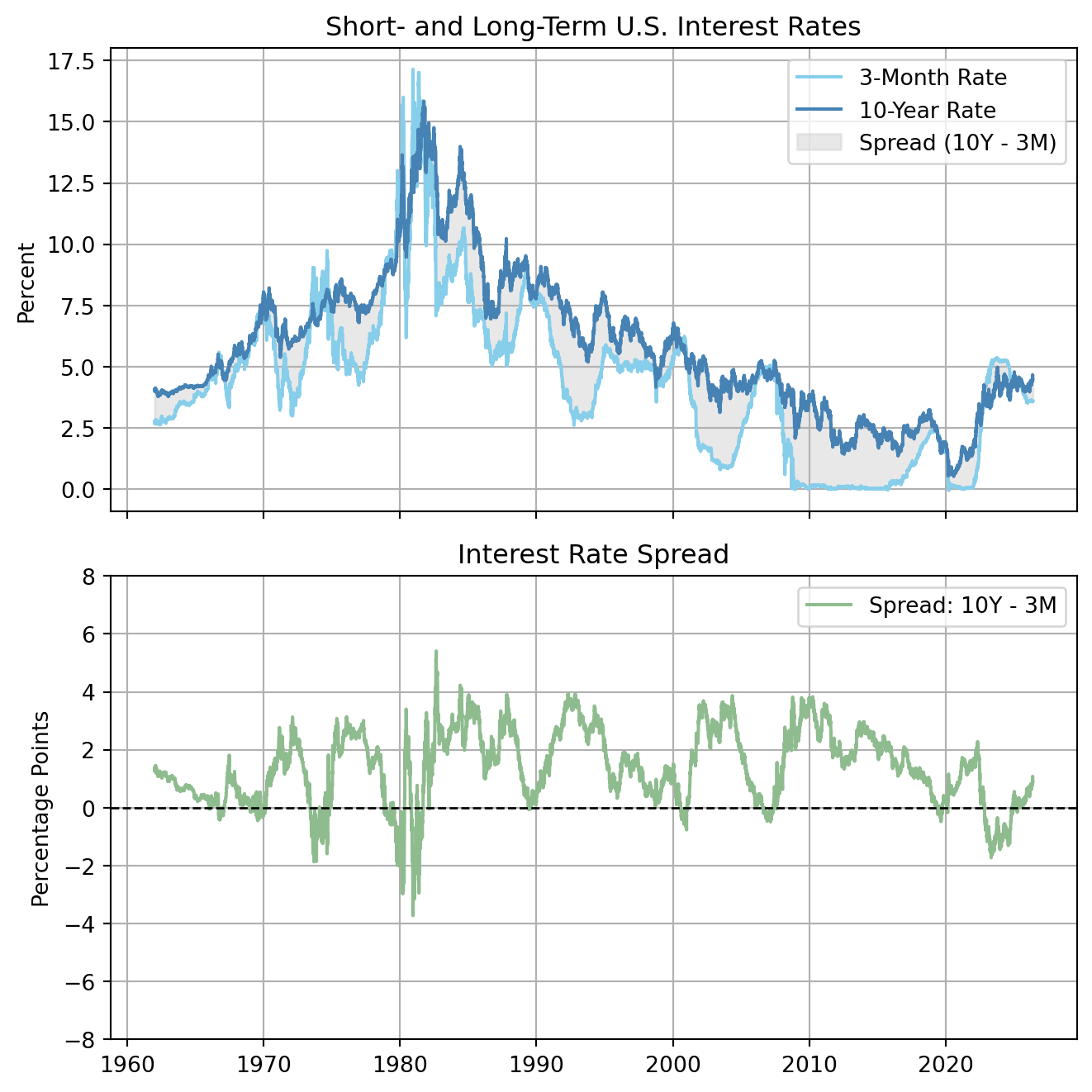
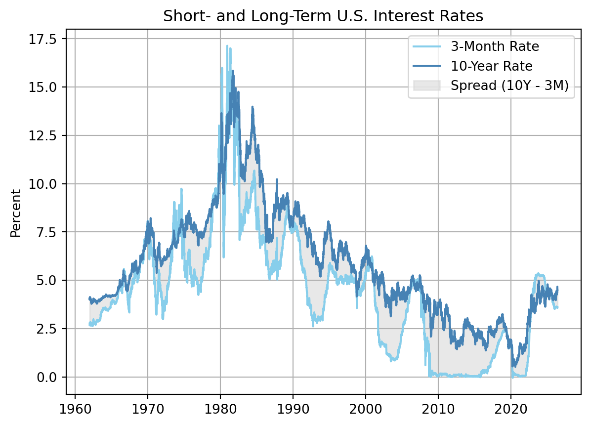
This, however, might create an important issue, if two nonstationary variables are linked by an economic equilibrium relationship in the long run, and we difference them mechanically, the long-run information contained in the levels of the variables may be removed. Take, for instance, income and consumption. Theory suggests both series grow over time, but may not be stationary on its own. Similarly, the prices of closely related financial assets, such as the interest rate on short vs long term bonds (Figure 6.1 top). Even though both series move over time, they do not drift apart indefinitely. Instead, they remain tied to one another by an equilibrium condition, so the spread (\(r_{10y} - r_{3m}\)) is relatively stable (Figure 6.1 bottom). That’s because they have a common stochastic trend. When this occurs, the series are said to be cointegrated.
Figure 6.1: US Treasury Maturity, 3-month vs 10-year
If we difference these variables blindly, they may lose meaningful long-run structure. Instead, we want a framework that tells us whether a long-run relationship exists. Cointegration is designed to address such cases, allowing us to work with variables that are individually nonstationary, while still capturing the possibility that they move together over time in a stable long-run relationship. Formally,
Cointegration
Let \(y_t\) and \(x_t\) be two time series such that:
\[
y_t ∼ I(1)
\]
\[
x_t ∼ I(1)
\]
are integrated of order 1. If there exists a constant \(\theta\) such that:
\[
u_t = y_t − \theta x_t ∼I(0)
\] is integrated of order zero, then \(y_t\) and \(x_t\) are cointegrated.
Although each series is nonstationary, a linear combination of them is stationary. The value of \(\theta\) defines the long-run relationship and is called the cointegrated coefficient.
In the example above, because both the short-term and long-term interest rates appear to have a strochastic trend, we would say that both series are integrated of order one, or I(1). The series are cointegrated if for some constant \(\theta\), the difference, \(r_{10y}-\theta r_{3m}\) is integrated of order zero, I(0).
6.2.1 Testing for cointegration
How can we test whether two nonstationary variables are cointegrated, i.e., if they share a stable long-run relationship? The Engle–Granger procedure gives us a simple and intuitive way to solve this issue. the procedure focuses on the estimated equilibrium error obtained from the long-run relationship. If this error is stationary, then the variables do not drift apart permanently and are said to be cointegrated. If the error itself remains nonstationary, then no stable equilibrium relationship exists between the variables.
The Engle–Granger approach is a simple two-step procedure:
1.- Estimate the long-run relationship between the variables.
For the interest rate example, define:
\[
r_t^{10y} = \alpha + \theta r_t^{3m} +u_t
\]
where:
\(r_t^{10y}\): 10-year Treasury rate
\(r_t^{3m}\): 3-month Treasury rate
\(u_t\): deviation from long-run equilibrium
The coefficient \(\theta\) measures the long-run association between short- and long-term rates. For example, if \(\hat{\theta}=0.75\) then, in the long run, a one percentage point increase in the short-term rate is associated with a 0.75 percentage point increase in the long-term rate.
The residuals are \(\hat{u}_t = \hat{r}_t^{10y}- r_t^{10y}\)
2.- Test the he residuals from that relationship for stationarity.
Apply stationarity tests to the residuals. If residuals are stationary, the evidence supports cointegration. If not, no evidence of cointegration.
Important: Because the residuals are not directly observed. They are estimated from a previous regression. The usual critical values are not strictly valid. In practice, it is better to use a dedicated cointegration tests.
The logic of the method follows directly from the definition of cointegration itself: if a linear combination of nonstationary variables is stationary, then the variables share a common stochastic trend and maintain a stable equilibrium relationship over time.
NoteExample
Show code
import pandas as pdimport numpy as npimport matplotlib.pyplot as pltimport seaborn as snsimport statsmodels.api as smfrom datetime import datetimefrom pandas_datareader import data as pdrfrom statsmodels.tsa.stattools import adfuller, kpss
a one percentage point increase in the short-term rate is associated with approximately a 0.85 percentage point increase in the long-term rate.
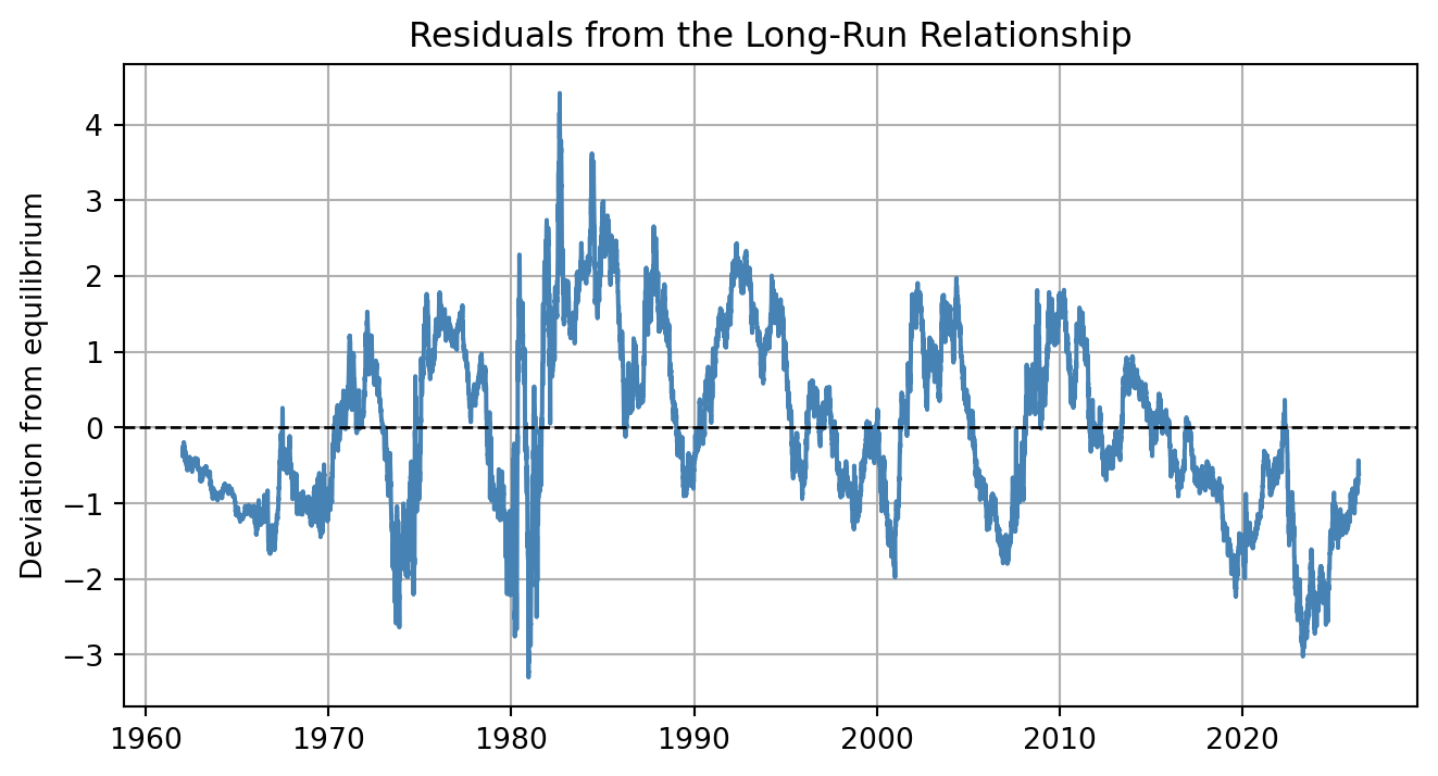
df["eg_residuals"] = eg_model.residplt.figure(figsize=(8, 4))plt.plot(df.index, df["eg_residuals"], color="steelblue")plt.axhline(0, linestyle="--", color="black", linewidth=1)plt.title("Residuals from the Long-Run Relationship")plt.ylabel("Deviation from equilibrium")plt.xlabel("")plt.grid(True)plt.show()
Do the residuals fluctuate around zero? do they drift permanently away?. The figure above suggests that the two interest rates may be cointegrated.
Step 2
adf_result = adfuller(df["eg_residuals"].dropna())print("ADF test on Engle-Granger residuals")print(f"Test statistic: {adf_result[0]:.4f}")print(f"p-value: {adf_result[1]:.4f}")print(f"Used lags: {adf_result[2]}")print(f"Observations: {adf_result[3]}")
ADF test on Engle-Granger residuals
Test statistic: -4.4283
p-value:        0.0003
Used lags:      21
Observations:   16062
Recall, the null hypothesis states the residuals have a unit root (non-stationary). Therefore, results suggest the residuals are stationary. However, the usual ADF critical values are not strictly valid, we then use Engle–Granger test, which also evaluates whether the residuals from the estimated long-run relationship contain a unit root. The null hypothesis states that the residuals are nonstationary, implying that no stable long-run equilibrium exists between the variables. Rejection of the null provides evidence of cointegration.
Engle-Granger cointegration test
Test statistic: -4.4285
p-value:        0.0016
Critical values:
[-3.89712109 -3.33650994 -3.04471372]
The results of the Engle–Granger test provide statistical evidence that the short-term and long-term interest rates are cointegrated. Although each interest rate appears to be individually nonstationary, the test suggests that a stable long-run equilibrium relationship exists between them. This finding is consistent with the idea that interest rates across maturities are linked through common market forces and expectations about future economic conditions.
Establishing cointegration tells us that a stable long-run equilibrium relationship exists between the variables. However, the Engle–Granger test does not explain how the system returns to equilibrium after temporary deviations occur. If short- and long-term interest rates drift apart in one period, what mechanism brings them back together? To answer this question, we require a model that combines short-run dynamics with long-run equilibrium adjustment. This leads naturally to the Error Correction Model (ECM).
6.2.2 Error Correction Model (ECM)
Cointegration implies deviations from equilibrium are temporary. Suppose: \(u_t =y_t−\theta x_t\) is the equilibrium error. If: \(u_{t−1}\) becomes large, then the variables should adjust in subsequent periods to restore equilibrium. The ECM allows short-run changes depend partly on past disequilibrium.
While without cointegration, we difference variables to remove trends, with cointegration we still difference the variables but preserve the long-run equilibrium information through the error correction term. As an example consider the simple model:
\[
\Delta y_t = \alpha + \delta \Delta x_t + \gamma u_{t-1} + \varepsilon_t
\] where: \(u_t =y_t−\theta x_t\) is called the Error Correction Term. \(u_{t-1}\) captures long-run disequilibrium, and \(\gamma\) captures the speed of adjustment.
In the example, suppose that the long-term rates become “too high” relative to short-term rates, then \(u_{t−1}>0\), future changes in rates should reduce this deviation, thus, \(\gamma\) is expected to be negative to indicate equilibrium correction. We want to estimate the simple model:
# Use the residuals from the Engle–Granger regression:df["ec_term"] = eg_model.residdf["ec_term_lag"] = df["ec_term"].shift(1)df["d_long_rate"] = df["long_rate"].diff()df["d_short_rate"] = df["short_rate"].diff()
The coefficient on the correction term is −0.0015 and it is statistically significant. The negative sign implies that when the long-term rate deviates from its equilibrium relationship with the short-term rate, subsequent changes in the long-term rate tend to move downward, helping restore equilibrium. The coefficient of −0.0015 indicates that approximately 0.15% of disequilibrium is corrected per day.
The coefficient 0.33 indicates that short-run changes in short-term interest rates are positively associated with contemporaneous changes in long-term rates. A one percentage point increase in the daily change of the short-term rate is associated with approximately a 0.33 percentage point increase in the daily change of the long-term rate.
ECM models may take several forms, provided they combine short-run dynamics expressed in stationary form with a lagged error correction term derived from a cointegrating relationship. Consequently, more flexible dynamic specifications such as SARIMAX models may also constitute Error Correction Models when they incorporate the equilibrium correction mechanism.
NotePractice
Mexican auto exports to the US and U.S. industrial production are closely connected through manufacturing supply chains and trade integration between both economies. Changes in U.S. industrial activity may influence the demand for imported vehicles and manufacturing components from Mexico, suggesting the possibility of a long-run relationship between these variables. In this exercise:
Estimate the cointegrating coefficient between the logarithm of Mexican auto imports and the logarithm of the U.S. industrial production index.
Apply the Engle–Granger cointegration test to determine whether a stable long-run equilibrium relationship exists between the variables.
If evidence of cointegration is found, explain its economic interpretation and proceed to estimate an Error Correction Model (ECM) to analyze how short-run deviations from equilibrium are corrected over time
6.2.3 Vector Error Correction Model (VECM)
The ECM in the example above treats the long-term interest rate as the variable that adjusts to restore equilibrium. However, in many economic systems, multiple variables may respond simultaneously to disequilibrium. In the case of interest rates, both short- and long-term rates may jointly participate in the adjustment process. More generally, when several endogenous variables are cointegrated, we require a framework capable of modeling their joint dynamics while preserving the long-run equilibrium relationship identified through cointegration. The Vector Error Correction Model (VECM) provides exactly this framework.
VAR model describes the joint evolution of several endogenous variables using their own lagged values:
This framework works well when the variables are stationary. However, when the variables are nonstationary and cointegrated, estimating a VAR in levels may lead to nonstandard behavior, while estimating a VAR in first differences may discard the long-run equilibrium information.
The VECM resolves this problem by combining short-run dynamics in differences with long-run equilibrium correction. In this sense, the VECM is simply a VAR reformulated to explicitly incorporate cointegration relationships. The VECM can be written as:
\[
\Delta Y_t = \Pi Y_{t-1} + \sum_{i=1}^{p-1} \Gamma_i \Delta Y_{t-i} + \epsilon_t
\] The term \(\Gamma_i \Delta Y_{t-i}\) captures short-run interactions among the differenced variables, analogous to the lagged differences appearing in standard dynamic models. The term \(\Pi Y_{t-1}\) contains the long-run information. The matrix \(\Pi\) can be decomposed as \(\Pi = \alpha \theta'\), where \(\theta\) contains the cointegration vectors that define the long-run equilibrium relationships among the variables and the matrix \(\alpha\) contains the adjustment coefficients that determine how strongly each variable responds to disequilibrium.
6.3 Conditional Heteroskedasticity
Traditional time series models such as ARIMA or SARIMA are designed to model and forecast the conditional mean of a series. These models generally assume
\[
Var(\varepsilon_t)= \sigma^2
\]
variance of the error term remains constant over time. It implies that the uncertainty remains stable, i.e., shocks have constant variability, and periods of tranquility and turbulence are equally likely over time.
One important characteristic of many financial time series, however, is that their variability changes over time. The concept of conditional heteroskedasticity:
\[
Var(\varepsilon_t | I_{t−1})=\sigma^2_t
\]
captures this feature. It implies that current volatility depends on past information. Here \(I_{t-1}\) represents information available up to period \(t−1\).
Moreover, in financial markets returns frequently display periods of persistent high and low volatility, this is known as volatility clustering. Even though the daily price change is difficult to forecast, the variance can be forecasted.
Models designed to capture this behavior are relevant for financial analysis because volatility is directly related to financial risk, portfolio management, derivative pricing, and investment decisions. The development of volatility models represented a major advance in econometrics allowing analysts to model not only the expected value of a process, but also the evolution of uncertainty itself. Two of the most influential models for this purpose are the Autoregressive Conditional Heteroskedasticity (ARCH) model and its extension, the Generalized ARCH (GARCH) model.
6.3.1 ARCH Models
The ARCH model, introduced by Robert Engle (Engle 1982), was the first major framework designed specifically to model time-varying variance. Consider a simple AR(1) autoregressive process:
\[
y_t = μ + \phi y_{t−1} + \varepsilon_t
\]
\(\varepsilon_t\) is modeled as being normally distributed with mean 0 and constant variance \(\sigma^2\), \(\varepsilon_t \sim \mathcal{N}(0,\sigma^2)\).
The ARCH model of order \(p\), denoted \(ARCH(p)\), instead assumes that the variance changes over time according to past shocks:
under this specification shocks in previous periods increase current volatility, both positive and negative shocks equally matter (squaring the residual removes the sign and measures the size of the shock). The term \(\omega\) captures the baseline level of volatility, while \(\alpha_i\) measures the impact of shocks in \(t-i\) on current variance. Thus, the ARCH model captures the short-run persistence of volatility.
The ARCH model can be applied to the error variance of any time series regression model with an error that has a conditional mean of 0, including autoregressions, and time series regressions with multiple predictors.
6.3.2 GARCH Models
Financial volatility is often highly persistent, meaning that shocks affect volatility for long periods, capturing this persistence solely through lagged squared errors becomes inefficient. ARCH models would require many lagged squared residuals. This creates several problems as too many parameters lead to
This motivated the development of the Generalized ARCH (GARCH) model, which extends ARCH by incorporating lagged conditional variances directly into the model.
this has become the standard workhorse model in financial econometrics.
\(\alpha_1\) Measures how strongly volatility reacts to new information. This component is often called the news effect.
\(\beta_1\) captures how persistent volatility is. If relatively large, volatility decays slowly, uncertainty remains elevated for many periods.
If \(\alpha_1 + \beta_1 < 1\) then shocks disappear rapidly (volatility quickly returns to normal levels), but if \[\alpha_1 + \beta_1 \approx 1\] volatility remains elevated for long periods.
NoteExample
Show code
import pandas as pdimport numpy as npimport matplotlib.pyplot as pltimport seaborn as snsimport statsmodels.api as smimport yfinance as yffrom pandas_datareader import data as pdrfrom statsmodels.tsa.stattools import adfuller, kpssfrom statsmodels.graphics.tsaplots import plot_acf, plot_pacffrom arch import arch_model
Note that we specified no lagged predictors in equation for the returns (why?), but can be generalized to an ARMA process.
model = arch_model(stock_pr['ret'], vol='GARCH', p=1, q=1, mean='Constant', dist='normal')model_result = model.fit(disp="off")print(model_result.summary())
                     Constant Mean - GARCH Model Results
==============================================================================
Dep. Variable:                    ret   R-squared:                       0.000
Mean Model:             Constant Mean   Adj. R-squared:                  0.000
Vol Model:                      GARCH   Log-Likelihood:               -1833.37
Distribution:                  Normal   AIC:                           3674.75
Method:            Maximum Likelihood   BIC:                           3695.57
                                        No. Observations:                 1347
Date:                Thu, May 28 2026   Df Residuals:                     1346
Time:                        10:11:39   Df Model:                            1
                                Mean Model
==========================================================================
                 coef    std err          t      P>|t|    95.0% Conf. Int.
--------------------------------------------------------------------------
mu             0.0784  2.286e-02      3.430  6.031e-04 [3.361e-02,  0.123]
                              Volatility Model
============================================================================
                 coef    std err          t      P>|t|      95.0% Conf. Int.
----------------------------------------------------------------------------
omega          0.0370  1.447e-02      2.556  1.058e-02 [8.632e-03,6.537e-02]
alpha[1]       0.1033  2.509e-02      4.118  3.827e-05   [5.414e-02,  0.153]
beta[1]        0.8615  3.227e-02     26.700 4.674e-157     [  0.798,  0.925]
============================================================================

Covariance estimator: robust
The two coefficients in the GARCH model (the coefficients on \(\alpha_1\) and \(\beta_1\)) are both individually statistically significant at the 5% significance level.
After estimating an ARCH or GARCH model, it is important to verify whether the model successfully captured the volatility dynamics. In ARIMA models, we assumed:
\[
\varepsilon_t \sim \mathcal{N}(0,\sigma^2)
\] which can rewritten as \(\varepsilon_t = \sigma z_t\), with \[
z_t \sim \mathcal{N}(0,1)
\]
The key innovation in GARCH is that \(\sigma\) is not constant but evolves over time, thus:
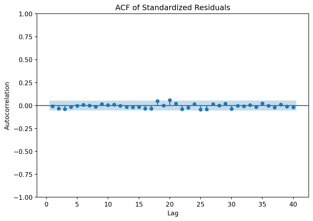
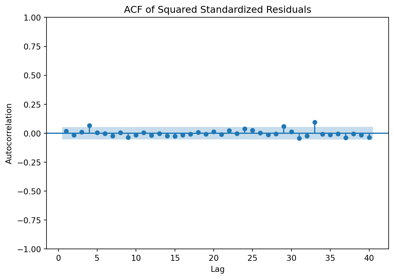
If the model is correctly specified, the standardized residuals should resemble white noise, squared standardized residuals should exhibit little autocorrelation.
Common diagnostic tools are:
Ljung–Box tests on squared residuals
ACF plots of squared residuals.
If significant autocorrelation remains, the model may still be misspecified.
Continue with the example:
Diagnostic checking
residuals = model_result.std_resid.dropna()plt.figure(figsize=(7, 5))plot_acf(residuals, zero =False, lags=40, alpha=0.05)plt.title("ACF of Standardized Residuals")plt.xlabel("Lag")plt.ylabel("Autocorrelation")plt.tight_layout()plt.show()
<Figure size 672x480 with 0 Axes>
print("\nLjung-Box Test Residuals:")print(acorr_ljungbox(residuals, lags=[10], return_df=True))
Ljung-Box Test Residuals:
    lb_stat  lb_pvalue
10  4.74798   0.907365
print("\nLjung-Box Test Squared Residuals:")print(acorr_ljungbox(sq_residuals, lags=[10], return_df=True))
Ljung-Box Test Squared Residuals:
     lb_stat  lb_pvalue
10  9.973145   0.442853
6.3.3 Forecasting volatility
A main advantages of ARCH and GARCH models is that they allow us to generate forecasts of future volatility. This is valuable in finance because investors, portfolio managers, and financial institutions are often more interested in forecasting future risk than forecasting returns themselves.
The logic behind volatility forecasting follows directly from the structure of the GARCH model. Recall that in a GARCH(1,1) framework, the conditional variance evolves dynamically according to past shocks and past volatility:
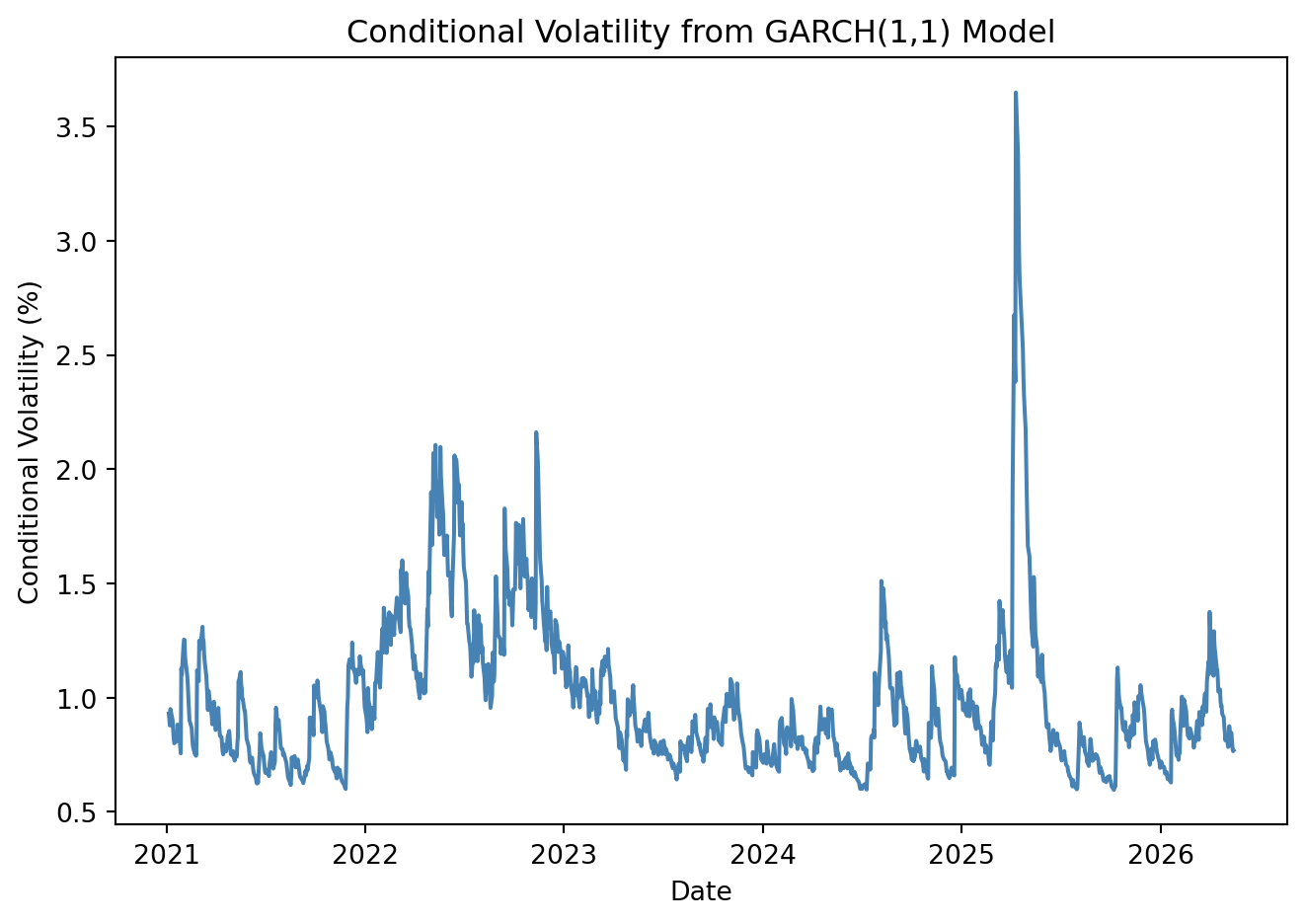
the fitted conditional volatility series can be extracted and visualized over time. This estimated volatility series reflects the model’s assessment of the level of market uncertainty at each point in time. Periods of financial stress typically appear as spikes in conditional volatility, while calmer market periods display lower estimated volatility.
The following code plots the estimated conditional volatility obtained from the fitted GARCH model:
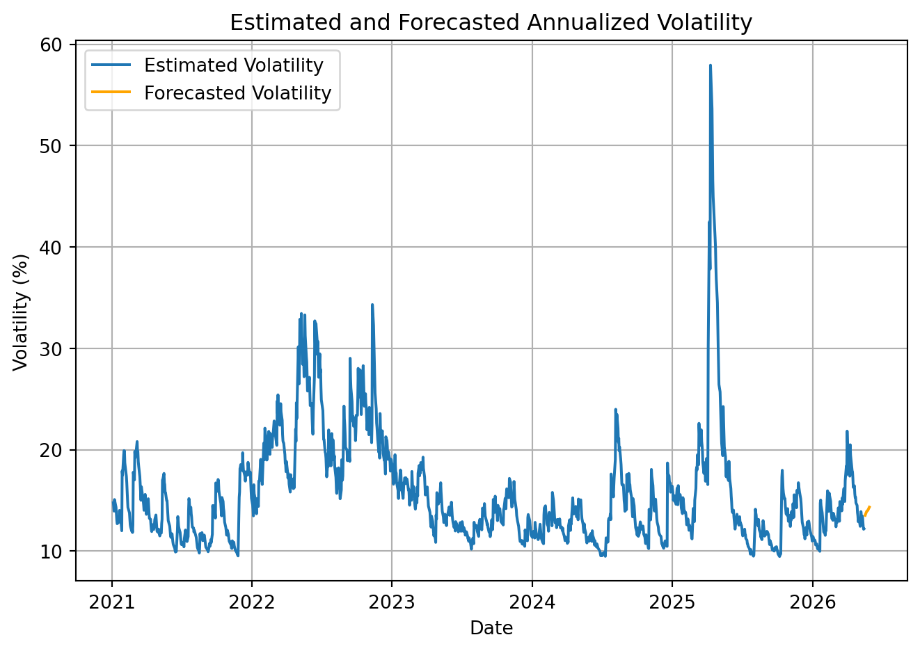
Once the model has been estimated, future volatility forecasts can be generated using the forecast method employed in earlier applications as the model recursively projects future conditional variances using the estimated GARCH dynamics.
The forecasted variances are then converted into standard deviations by taking the square root: \[
\hat{\sigma}_{t+h} = \sqrt{\hat{Var}(\varepsilon_{t+h})}
\]
Because daily volatility is often difficult to interpret directly, the forecasts are annualized using 252 as the number of trading days in a year. Annualized volatility provides a more intuitive measure of financial risk and facilitates comparisons across assets and time periods.
The forecasted daily and annualized volatility values are summarized in a table:
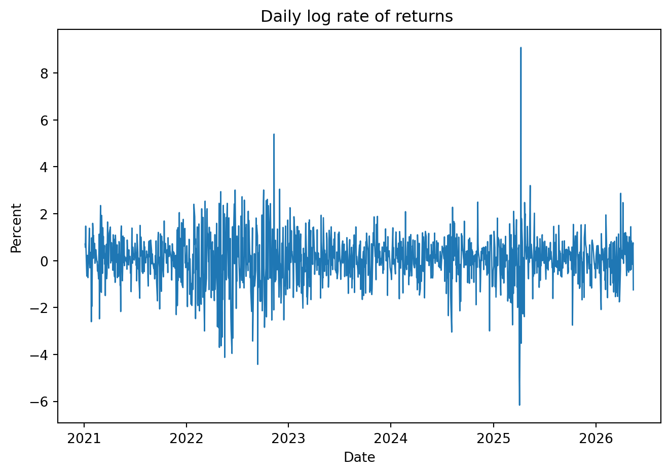
The Wilshire 5000 Total Market Index (^W5000) represents one of the broadest measures of the U.S. equity market and therefore provides a useful benchmark for analyzing aggregate market volatility, particularly given the strong interconnectedness between U.S. and Mexican financial markets. Because the index reflects the performance of thousands of publicly traded firms, periods of financial stress and market uncertainty are often associated with persistent changes in volatility, making the series well suited for estimation using a GARCH(1,1) model.
Using daily log returns from the Wilshire 5000 index (^W5000), complete the following:
Determine whether the return series exhibits evidence of conditional heteroskedasticity. Estimate an appropriate GARCH model, interpret its parameters, and evaluate whether the model adequately captures the volatility dynamics through diagnostic checking.
Generate volatility forecasts for the next 10 trading days. Interpret the behavior of the forecasts and explain whether the model suggests increasing, decreasing, or persistent future market uncertainty.
Engle, Robert F. 1982. “Autoregressive Conditional Heteroscedasticity with Estimates of the Variance of United Kingdom Inflation.”Econometrica 50 (4): 987. https://doi.org/10.2307/1912773.